The math and the papers
The bot's central problem is small to state. Given a cycle of pools, how much of the starting token should we put in so that the profit is as large as it can be? This page collects the reading that led to the answer and the derivation. It follows the answer from my own first attempt, which was in the right ballpark, to the answer in the cyclic arbitrage paper (Cyclic Arbitrage in Decentralized Exchanges, listed below), which made it exact, and then from Uniswap V2 to V3.
Reading list
- Cyclic Arbitrage in Decentralized Exchanges
Y. Wang, Y. Chen, H. Wu et al. · 2021 (arXiv 2105.02784, v3 Jan 2022)
Studied closely. It is the source of the idea that a chain of pools can be collapsed into one virtual pool with a closed-form optimal trade. The bot's `Path` class cites it.
- Uniswap v3 Core
H. Adams, N. Zinsmeister, M. Salem, R. Keefer, D. Robinson · 2021
With the v3-core contracts, the source for the off-chain V3 swap reimplementation.
- Liquidity Math in Uniswap V3
A. Elsts · 2021
Companion reference for V3 liquidity and tick math.
- An Analysis of Uniswap Markets
G. Angeris, H.-T. Kao, R. Chiang, C. Noyes, T. Chitra · 2019 (arXiv 1911.03380)
Background on constant-product market behavior.
Reference code and documentation:
- Uniswap v2-core
- Uniswap v3-core
- dYdX Solo Margin (flash loans on Ethereum)
- DODO flash loans (BNB Chain and Polygon)
- Flashbots documentation (bundles and relays)
The two-pool case: my first answer
Before I found the cyclic arbitrage paper, I worked the two-pool problem out on paper myself. The idea is simple. Two pools quote the same pair at different prices, so I buy the token where it is priced low and sell it into the other pool, where it is priced high. Each trade moves the price against me, so the profit peaks at the trade size where the two pools quote the same price again.
Setting it up
Call the token I start with, and get back at the end, . Call the token in the middle . Two pools trade this pair:
- The first pool holds of and of .
- The second pool holds of and of .
The names come from my notes. The letter is what goes into a pool when I trade, and is what comes out. I will carry one example through every step: the first pool holds 250 and 1,000 , and the second holds 500 and 2,000 .
Step 1: the price of . The price of one in a pool is the amount of in the pool divided by the amount of . In the first pool that is . In the second pool it is . So is priced low in the first pool and high in the second. I buy it in the first pool and sell it in the second.
Step 2: the rule a pool follows. When I trade, a pool's two reserves change, but the two reserves multiplied together stay the same. Ignoring the fee for now, call that number :
Step 3: buy of from the first pool. The pool now has of . Its two reserves must still multiply to , so:
Divide both sides by to get the amount of the pool holds afterwards:
In the example, buying leaves 500 in the pool, so it holds . It started with 250, so I paid in 250.
Step 4: sell the same into the second pool. That pool now has of , and by the same reasoning it holds of . In the example it has 1,000 and . It started with 2,000, so I took out 1,000. I paid in 250 and got back 1,000.
Step 5: the new prices. The price is divided by again. Dividing a fraction by something puts that something in the bottom a second time, so:
In the example both come out to 1 (500 divided by 500, and 1,000 divided by 1,000).
Step 6: the best trade is where the two prices meet. While is still priced lower in the first pool, buying a little more still makes money. If it has become priced lower in the second pool, I bought too much. So the best makes the two prices equal:
Solving for x
Step 7: take the square root of both sides. The square root of a fraction is the square root of the top over the square root of the bottom, and the square root of something squared is the something itself. So:
Step 8: multiply across. Multiply both sides by and by :
Step 9: open the brackets.
Step 10: gather the terms on the left. Add to both sides and subtract from both sides:
Step 11: pull out the common .
Step 12: divide both sides by the bracket.
Check it with the example. The square roots are and , so . That is the trade from step 3.
What I pay in
Step 13: what I pay in. From step 3, what I pay in is the change in the first pool's reserve:
To get this in terms of the reserves alone, I need to replace . I do it in three parts: simplify , use it to simplify the fraction, then subtract .
Step 14: simplify . From step 12, is a fraction. Call its top and its bottom :
So I want . You cannot subtract a fraction from a whole number directly. It works like : write the 3 as first, and then .
14a. Give the same bottom. Multiplying the top and bottom by changes nothing, because :
14b. Subtract. The bottoms match now, so only the tops combine:
14c. Write out the top. First, . Then subtract all of . The minus sign applies to both parts of , so both signs flip:
14d. Cancel. and are the same amount with opposite signs, so they cancel and leave:
14e. Factor. Both parts contain , so pull it out:
Check it with the example, where , and . The bottom is 1,500. The top is . The fraction is , which matches .
Step 15: use it in the fraction. Now divide by that result. Dividing by a fraction means multiplying by its flip:
15a. Cancel one . Write . One of them cancels with the on the bottom:
15b. Open the bracket. and :
In the example this is , the the pool holds afterwards, as in step 3.
Step 16: subtract . This is another fraction minus a whole number. Give the bottom :
Step 17: cancel and finish. Since , the terms and cancel. Also . That leaves:
In the example that is , the 250 I paid in at step 3.
What my notes had
The steps above are the tidy version, worked out afterwards. My scratch notes were messier. I set up the equal-price condition with the fee in it, boxed the equation, and pencilled the optimal amount in below it. With and the fee factors (0.997) on the input of each pool, the pencilled line reads:
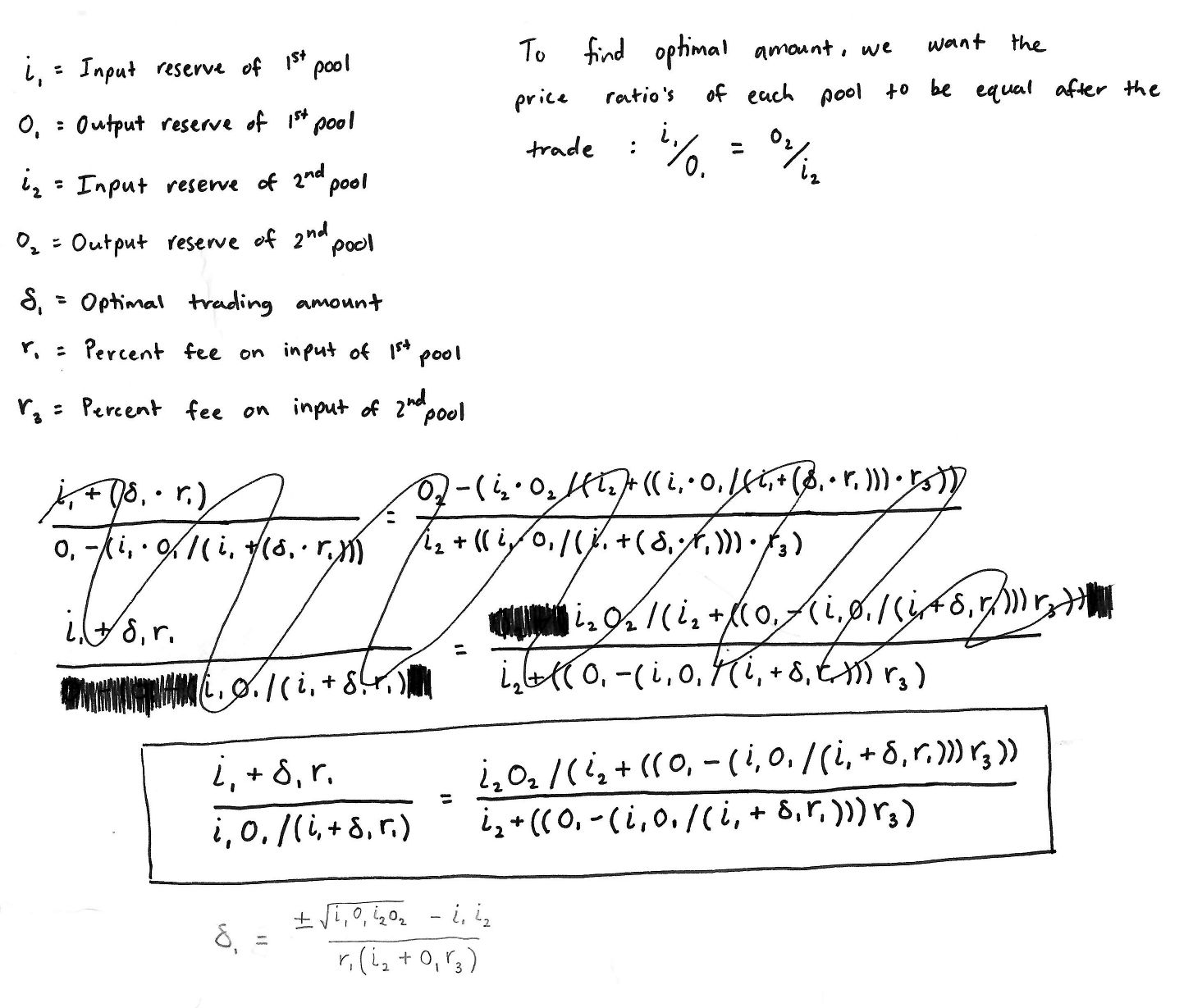
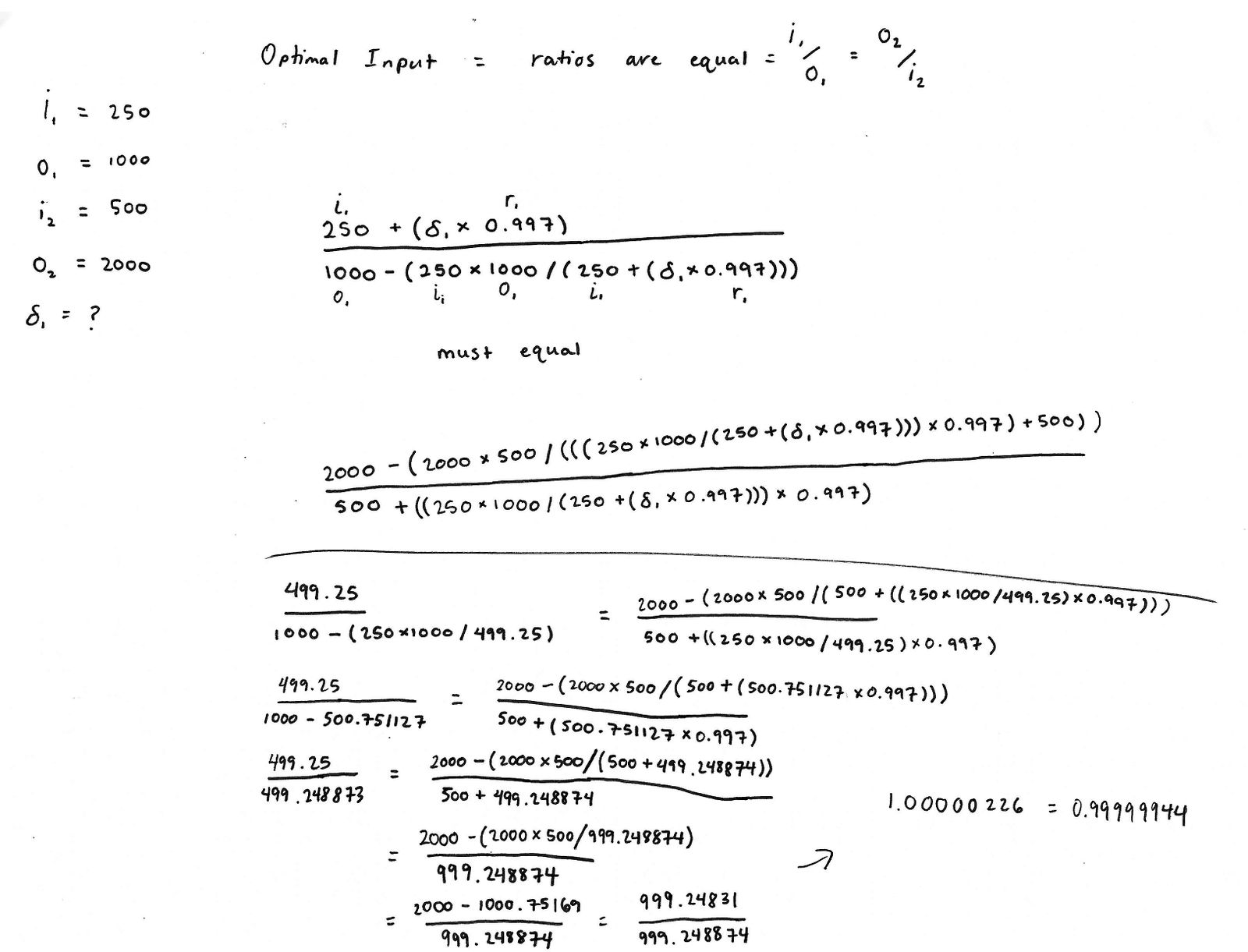
It is close, but not exact. For the example it gives 251.25, and the true best input is 250.25. The profit differs only in the fourth decimal place, 747.7432 against 747.7462, so the trade was nearly as good. With a fee, the profit peaks where the marginal prices, fee included, balance, and that is not quite where the reserve ratios are equal.
What the first bot did
The notes were not what ran. The function that turned them into code is calculateAmountToBuy in zzz-the-josh-bot, and it was a rougher implementation. It did not take the square root. It multiplied the equal-price condition out instead, which gives a quadratic:
The function then worked out both of its roots and kept whichever was in range:
This is where the edge cases came from. Squaring adds a second, false root, the one where the two prices are equal and opposite. So the code had to handle every combination: both roots negative, both in range, both zero, both too large. It also divides by , so two pools with the same constant broke it, and the code stopped there with a TODO. The square-root form from the steps above has one root and no such division. On 20,000 random pairs of pools it matches one of the code's two roots every time, and it still works when .
The fee was not in this formula at all. The router's getAmountIn added it afterwards, when the trade was priced. So the first bot was in the right ballpark, and no more than that. The cyclic arbitrage paper is what made it exact.
What the cyclic arbitrage paper added: a virtual pool
The paper closes both gaps: the fee goes inside the formula, and the answer is exact for any number of pools, not only two.
Wang et al. set the problem up with their own notation, which I use from here. is the reserve of token in the pool that pairs it with . The fee factors are on a pool's input and on its output, so on Uniswap V2 and . A swap of of for of in a pool with reserves and obeys , which solves to:
Their insight is that a whole chain of pools can be replaced by one virtual pool. For a cycle , fold the first pools into a virtual pool with reserves and . This is their Algorithm 1. Start with and , then for each next pool :
The closing pool, between and , then merges with the virtual pool into a single pool with reserves:
The whole cycle now behaves like one trade through a pool with reserves and . Its output is , so the profit is that minus . It starts at zero, climbs, peaks and falls, and at the peak its slope is zero, which gives the optimal input:
A profit exists only when the slope at is positive, which is the same as the product of the exchange rates around the cycle, net of fees, being greater than one. That is the test isValueExtractable runs before any real work.
For two pools, and the virtual pool is just the first pool. My symbols map onto the cyclic arbitrage paper's as , , and , and the paper's answer becomes:
Without a fee this is identical to what I found on my own. With the fee it has the same denominator, and one extra factor of on the square root. That factor is the part my equal-price shortcut missed.
The example from my notes, a first pool of 250 and 1,000 and a second pool of 500 and 2,000, comes out as follows. With no fee, is 83.33 and is 1,333.33, so the best input is , for a profit of 750. With the 0.3% fee, is 83.50 and is 1,331.997, and the best input moves to 250.25, for a profit of 747.75. A brute-force search over every input size lands on the same numbers.
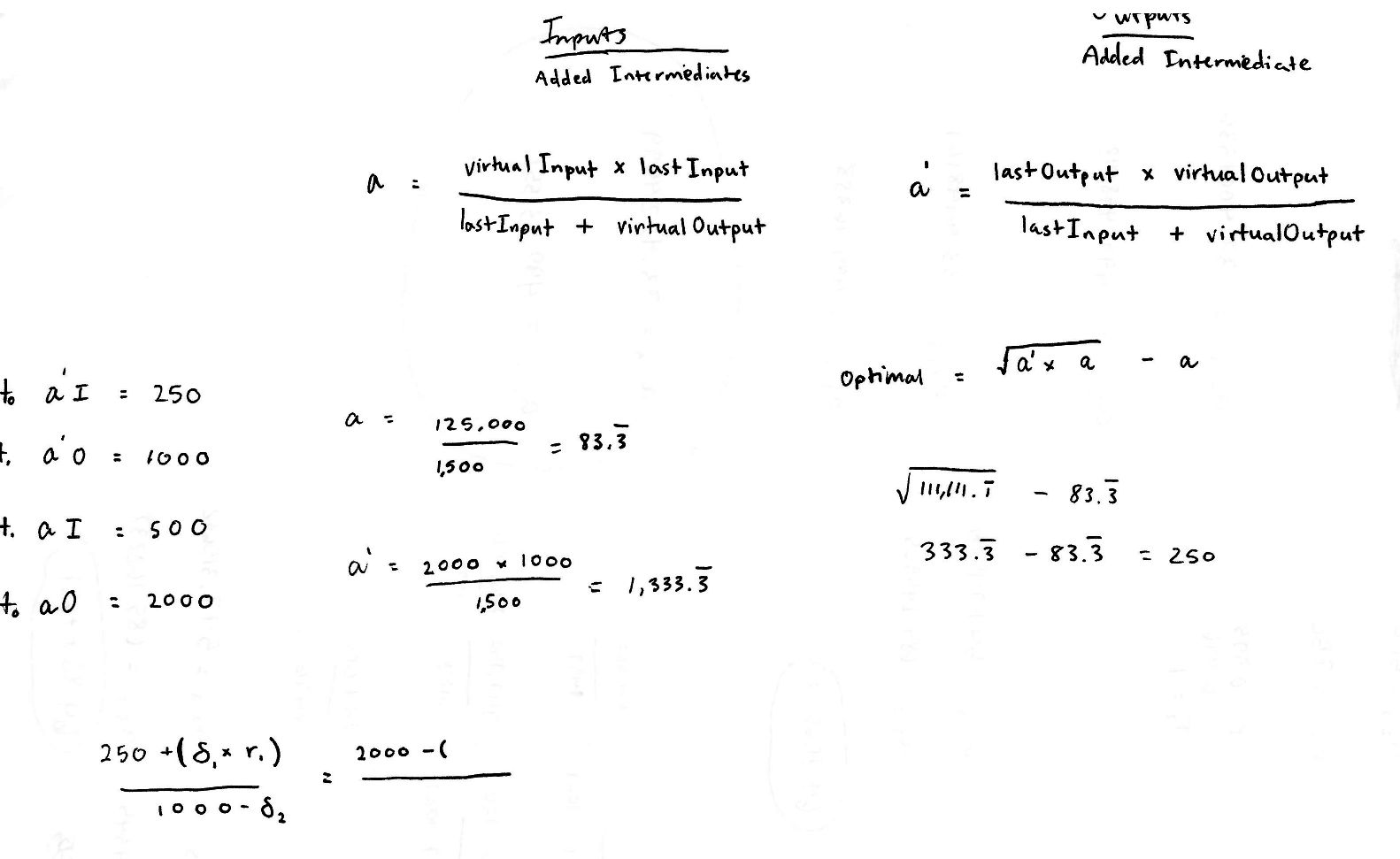
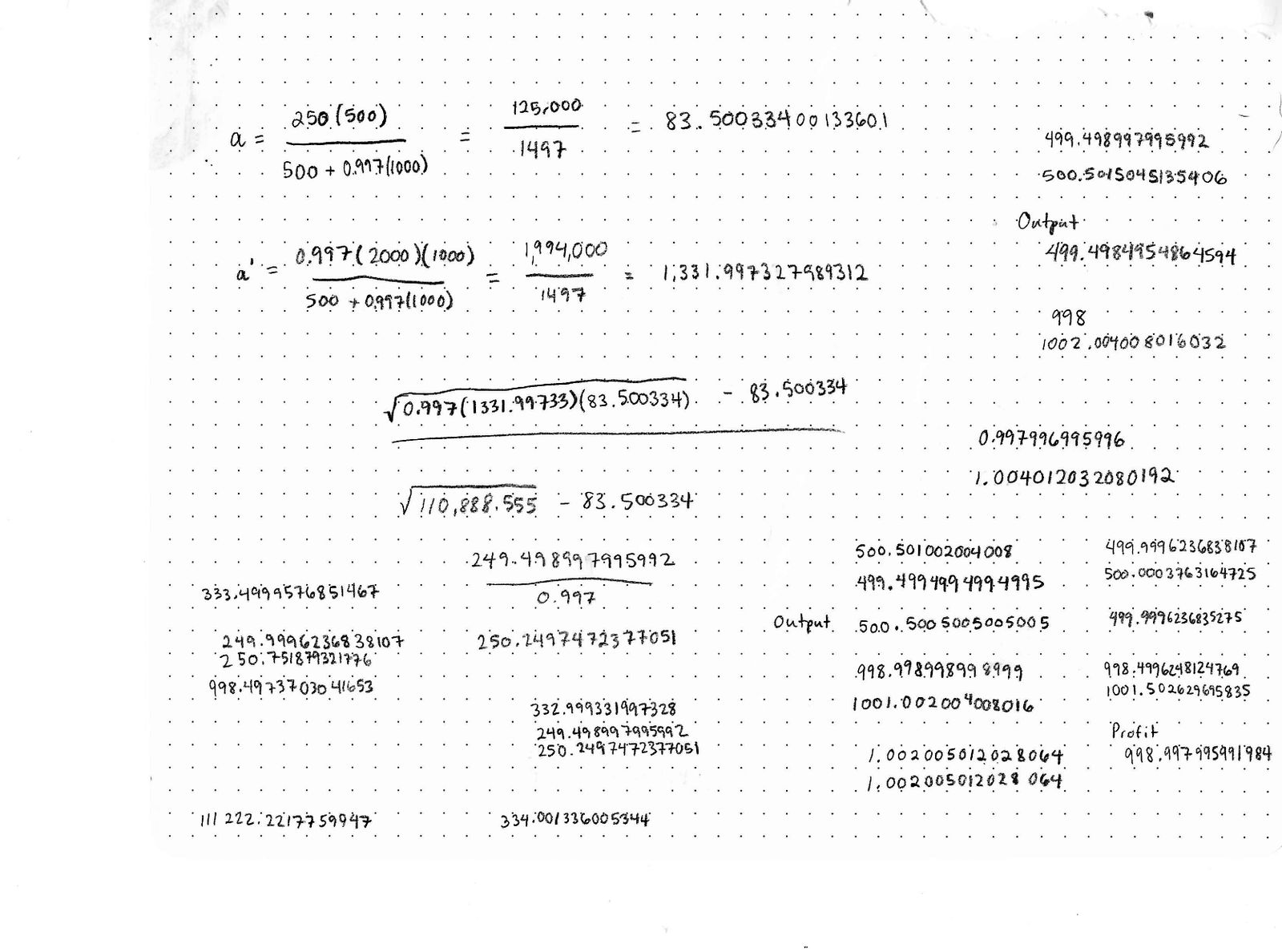
For a path of more pools, fold in one pool at a time with the two update rules above. A three-pool example agrees with brute force too, to the hundredth.
How the code followed
The three bots show the same arc as the notes, from a close approximation to the exact answer.
| Bot | Where | How it sized the trade | Result |
|---|---|---|---|
| First bot, 2022 | zzz-the-josh-bot, Arb.js | Solved the fee-free equal-price condition as a quadratic. The fee was not in the formula, and the router added it afterwards. | In the right ballpark, not exact. |
| Second bot, 2022 | zzz-do-not-go-gentle, util.js | Built the cyclic arbitrage paper's virtual pool and used its closed form, with the fee inside the formula. | Exact. |
| JamBot, 2023 | jam-bot, Path.calculateOptimalTradingVolume | The same fold and formula, rewritten in Java and extended to Uniswap V3 by stepping through ticks. | Exact within each V3 range. |
The Java implementation of this step is Path.calculateOptimalTradingVolume in jam-bot, and the method that decides whether a path is worth evaluating at all is isValueExtractable in the same class.
Pool 1
250 → 1,000
Pool 2
500 → 2,000
Virtual pool
Start with pool 1: its reserves become a and a′.
Input
0.00
Output
0.00
Profit
0.00
Uniswap V3: concentrated liquidity
V3 changes the curve. Liquidity is provided inside price ranges, so within one range a pool behaves like a V2 pool with larger virtual reserves, and the moment the price leaves the range the behavior changes. The optimizer therefore works in steps: solve as if the current range lasts forever, check whether the answer crosses the next initialized tick, and if it does, swap exactly up to that tick, update the pool's state, and solve again. Repeat until the answer stays inside a range.
The off-chain code has to match the contract exactly, because the contract is the final judge of every trade. The V3 swap math was therefore ported to integer arithmetic in Java, about 1,100 lines written in five commits between May 17th and June 3rd, 2023, the day the V3 executor went on chain. Pseudo-code for the swap loop (the SwapState and StepComputations structures) was transcribed by hand before any of it was written as code.
You spend
$0
ETH received
0.00
Price now
$2,040
Ticks crossed
0
What we did not get to
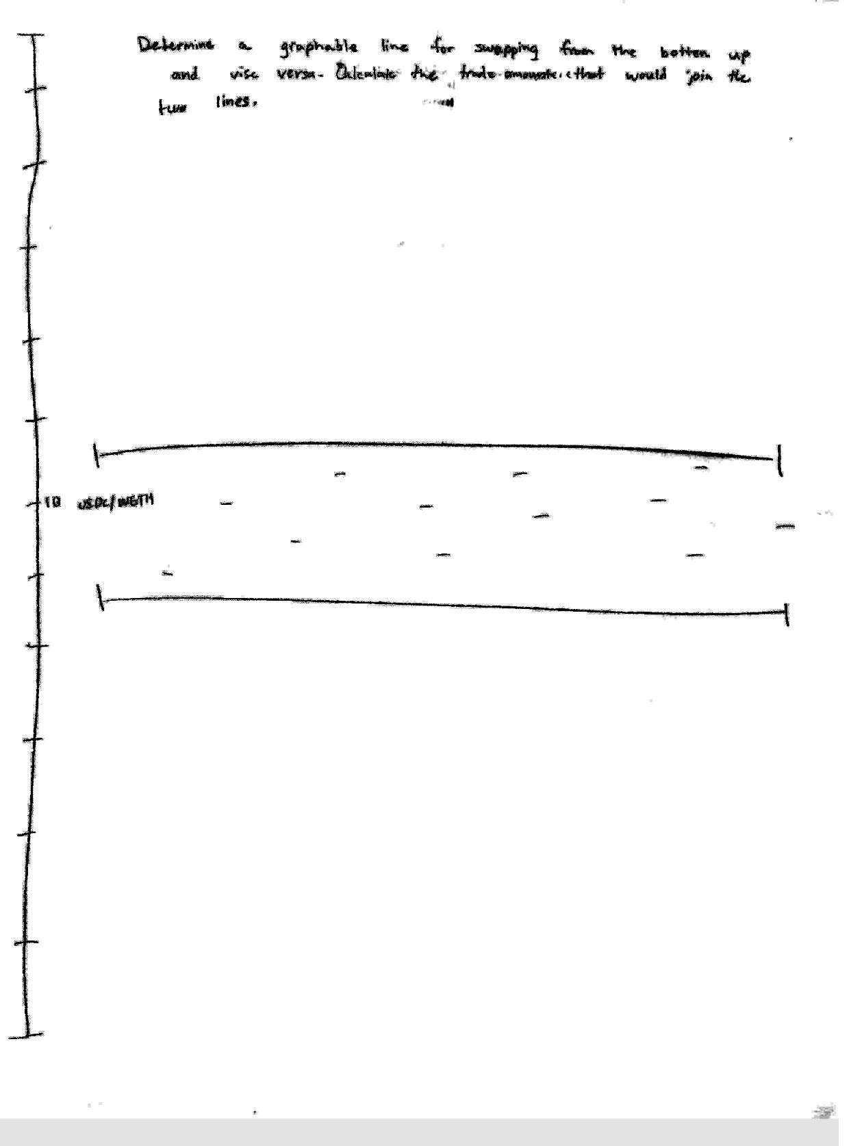
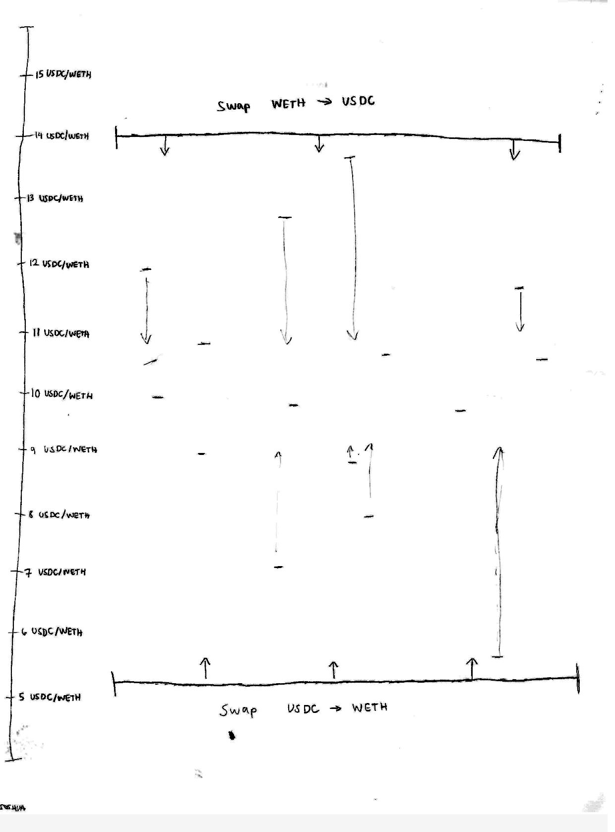
The multi-pool version of the problem: instead of one path at a time, look at every pool of a token pair at once and find the single price at which all of them are in balance. It is a convex optimization problem, and the scratch notes call it "a graphable line". We worked out the idea and never built it.
These notes sketch it as a graph. Price levels run up a vertical axis, swaps from the bottom are stacked against swaps from the top, and the trade that joins the two lines is the answer.
The research that formalises it is where we would start if we picked the project up again:
- G. Angeris, A. Agrawal, A. Evans, T. Chitra and S. Boyd, Constant Function Market Makers: Multi-Asset Trades via Convex Optimization (2021). Shows that choosing a trade across many assets and pools is a convex optimization problem.
- G. Angeris, T. Chitra, A. Evans and S. Boyd, Optimal Routing for Constant Function Market Makers (2022). Routes an order across a network of pools, with finding an arbitrage as a special case.